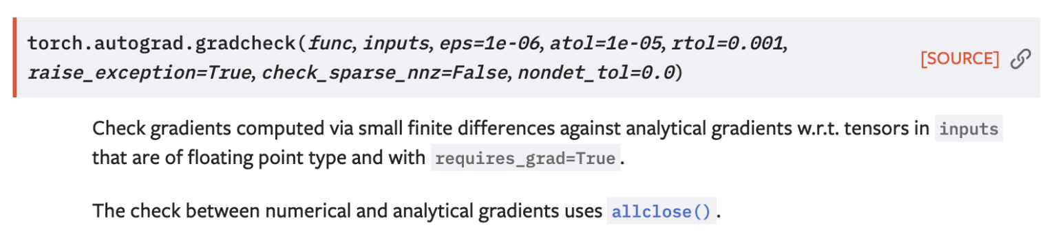
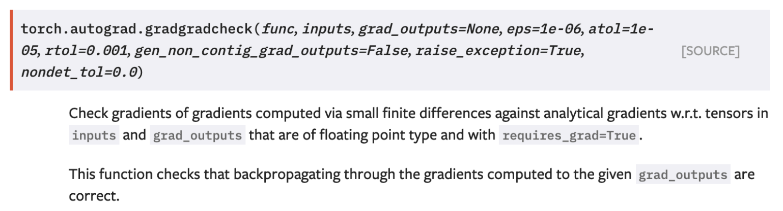
To minimizing the loss function, we should computing gradients, <u>in practice</u>, always use analytic gradient (exact, fast, error-prone), but check implementation with numerical gradient (approximate, slow, easy to write). This is called a gradient check. There are gradcheck and also gradgradcheck function in pytorch!

Gradient Descent

Iteratively step in the direction of the negative gradient (direction of local steepest descent).

# Vanilla gradient descent
w = initialize_weights()
for t in range(num_steps):
  dw = compute_gradient(loss_fn, data, w)
  w -= learning_rate * dw

Hyperparameters:

• Weight initialization method
• Number of steps
• Learning rate (step size)

Batch Gradient Descent

Because we are training a large dataset, the loss function and it gradient are:

$L(W)=\frac{1}{N} \sum_{i=1}^N L_i(x_i,y_i,W)+\lambda R(W)$

$\nabla_WL(W)=\frac{1}{N} \sum_{i=1}^N \nabla_WL_i(x_i,y_i,W)+\lambda \nabla_WR(W)$

However, full sum expensive when N is very very large!

Stochastic Gradient Descent (SGD)

Rather than computing a sum over the full training dataset, instead we will approximate this loss function and approximate the gradient by drawing small samples of our full training dataset. The typical sizes of these small sub samples are called minibatch (32 / 64 / 128 common). Then we modify our algorithm.

# Stochastic gradient descent
w = initialize_weights()
for t in range(num_steps):
  minibatch = sample_data(data, batch_size)
  dw = compute_gradient(loss_fn, minibatch, w)
  w -= learning_rate * dw

Hyperparameters:

• Weight initialization
• Number of steps
• Learning rate
• Batch size: how many elements should be in each minibatch
• Data sampling

Why we called this algo Stocastic?

Think of loss as an expectation over the full data distribution $p_{data}$. Then, approximate expection via sampling.

$\begin{aligned} L(W) &= \mathbb{E}_{(x,y)\sim p_{data}}[L(x,y,W)] + \lambda R(W) \\ &\approx \frac{1}{N} \sum_{i=1}^N L(x_i,y_i,W)+\lambda R(W) \end{aligned}$

$\begin{aligned} \nabla_W L(W) &= \nabla_W \mathbb{E}_{(x,y) \sim p_{data}}[L(x,y,W)] + \lambda \nabla_W R(W)\\ &\approx \sum_{i=1}^N \nabla_W L_W(x_i,y_i,W) + \nabla_W R(W) \end{aligned}$

However, there also some situations that this basic version of SGD might run us into trouble.

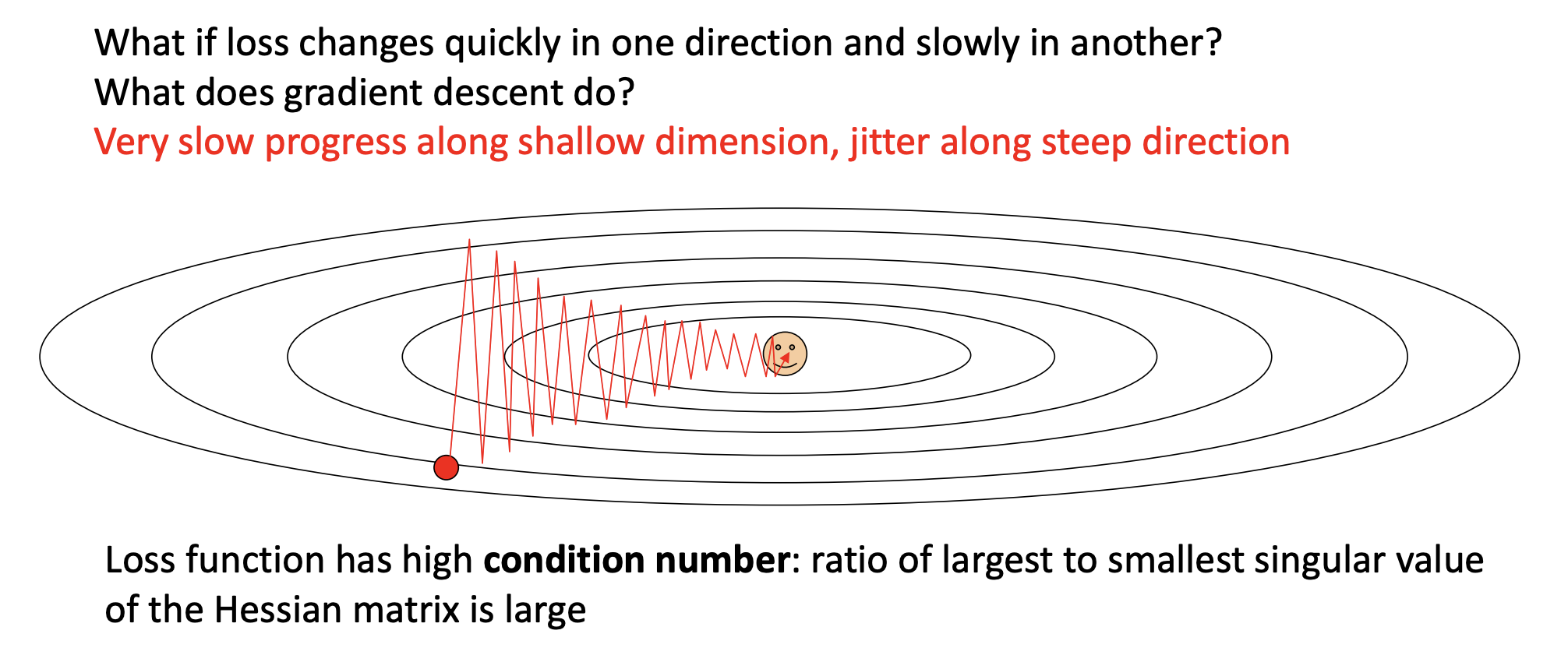
• Hessian 矩阵 (Hessian Matrix)：在优化中，Hessian 矩阵（记为 H）是损失函数的二阶导数矩阵。它描述了函数在某一点的局部曲率信息。具体来说：
  • Hessian 矩阵的特征向量（Eigenvectors）指向损失函数曲面的主曲率方向。
  • Hessian 矩阵的特征值（Eigenvalues）表示在这些主曲率方向上的曲率大小（二阶导数）。一个大的特征值意味着在那个特征向量方向上的曲率大（函数变化陡峭），一个小的特征值意味着在那个方向上的曲率小（函数变化平缓）。
• 奇异值 (Singular Values)：对于实对称矩阵（Hessian 矩阵通常是实对称的），其奇异值（Singular Values）就等于其特征值的绝对值。所以这里讨论 Hessian 的奇异值，本质上就是在讨论其特征值的绝对值。
• 条件数 (Condition Number)：矩阵的条件数通常定义为该矩阵最大奇异值与最小奇异值的比值。即 κ(H) = σ_max(H) / σ_min(H)。

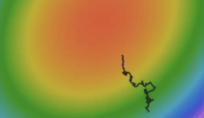
1. What if the loss function has a local minimum or saddle point?

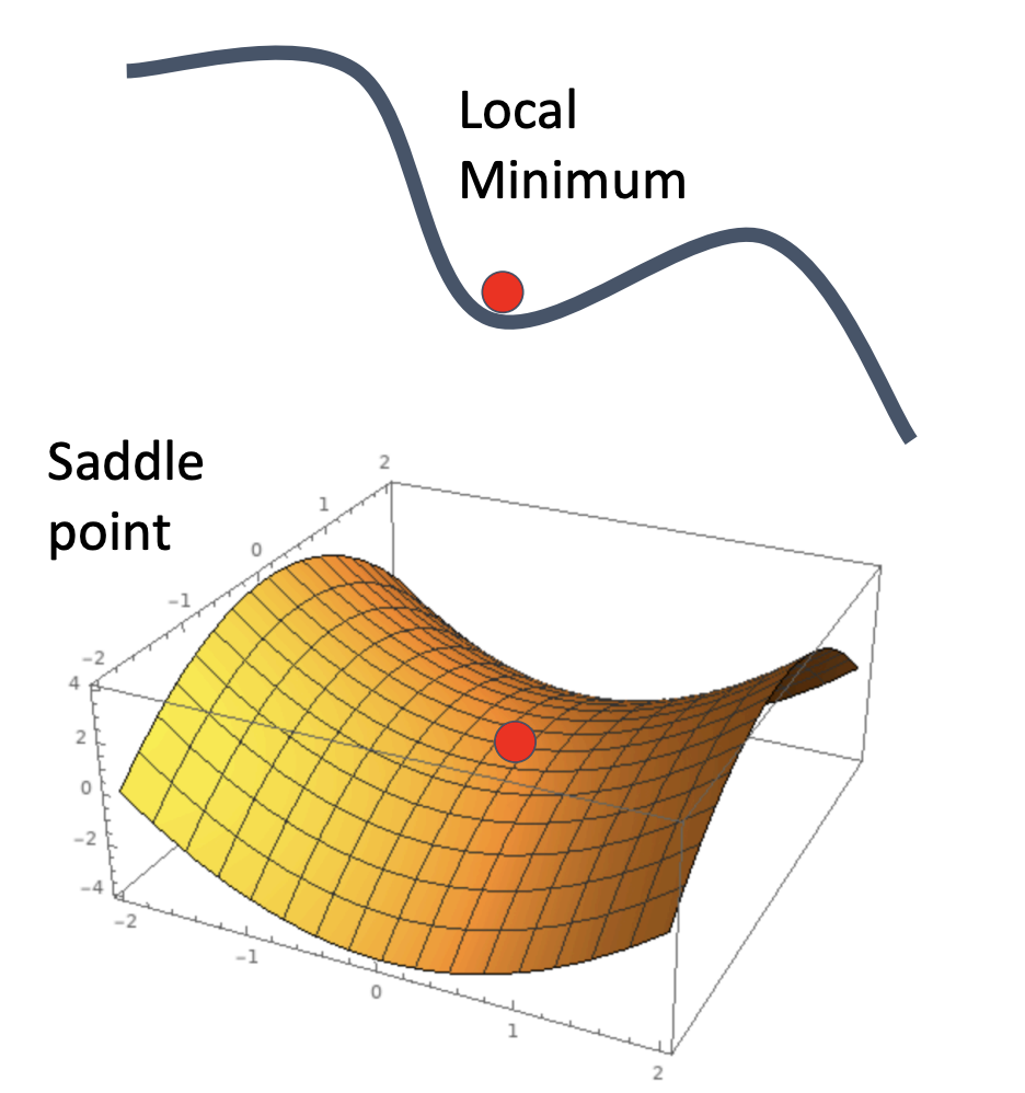
Zero gradient, gradient descent gets stuck!

1. For stochatic part, our gradients come from minibatches so they can be noisy!

SGD + Momentum

So, to address these kinds of problems, instead of using the simple vanilla gradient descent, we use SGD + Momentum.

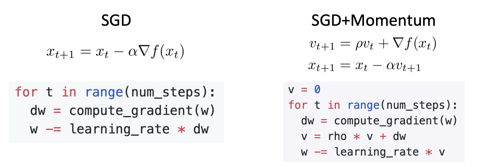
• Build up "velocity" as a runing mean of gradients
• Rho gives "friction"; typically rho = 0.9 or 0.99
• Adding Momentum is like let a ball rolling down the hill, at the zero gradient point, it still has velocity to move it up!

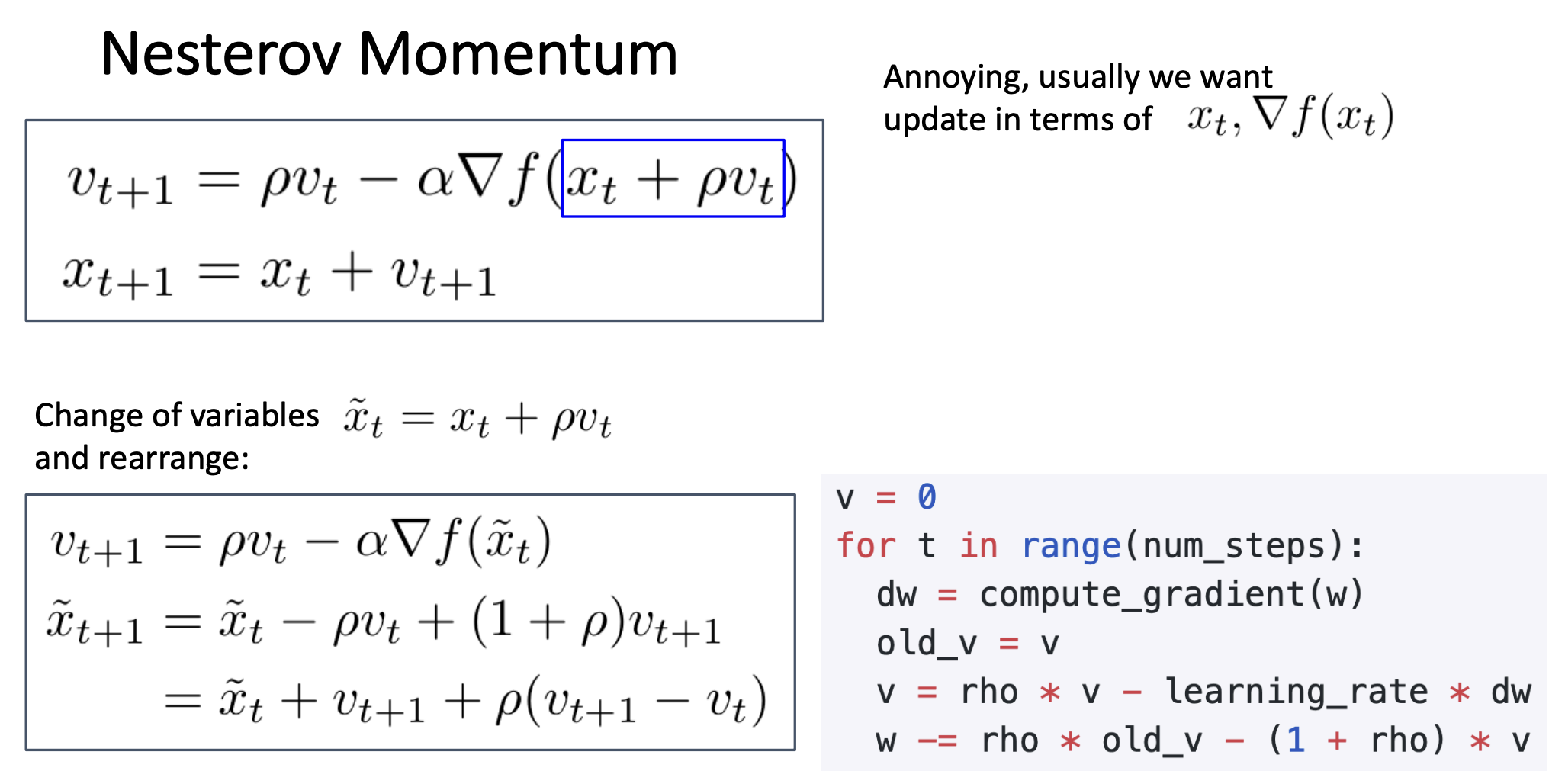
Nesterov Momentum

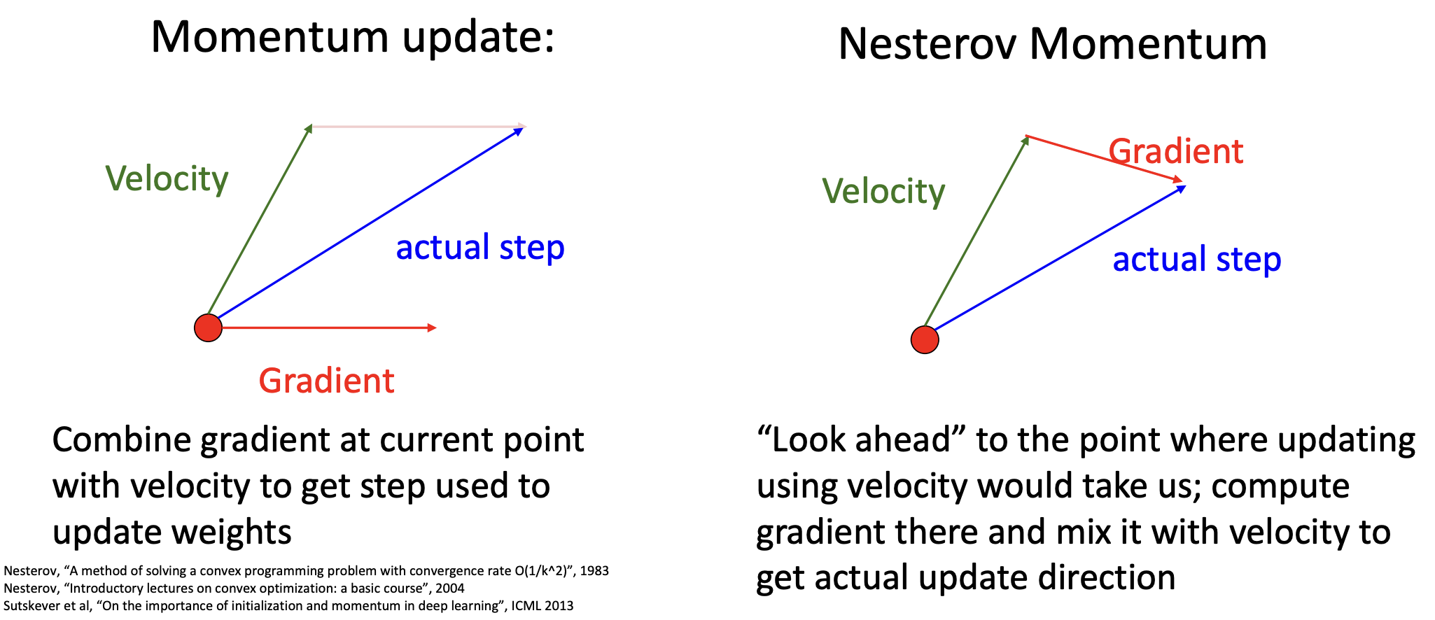
• Nesterov 动量在当前位置θ看速度v，预判“如果我按当前速度滑一步，我会滑到哪里 (θ_lookahead)？”，然后它在那个预判的位置 (θ_lookahead)看梯度，思考“如果我真滑到那里了，从那个地方我该怎么走？”。
• 这个前瞻的梯度g包含了关于即将到来的地形变化的信息。如果根据当前速度v滑下去会冲上一个坡（导致损失增加），那么在前瞻点θ_lookahead计算出的梯度g就会指向阻止这个上冲的方向。
• 当这个前瞻梯度g被用来更新速度v时，它有效地提前施加了刹车或进行了转向。它不是在参数已经冲上坡后才被拉回来，而是在冲上坡之前就根据预判调整了方向。

AdaGrad

A different way to address the problems of SGD. Rather than tracking the historical average of gradient values, we're going to keep track of a historical average of squares of gradient values. That is, added element-wise scaling of the gradient based on the historical sum of squares in each dimension. "Per-parameter learning rates" or "adaptive learning rate".

grad_squared = 0
for t in range(num_steps):
  dw = compute_gradient(w)
  grad_squared += dw * dw
  w -= learning_rate * dw / (grad_squared.sqrt() + 1e-7)

So, for the situation 1 in SGD, what happens with AdaGrad?

• Progress along "steep" directions is damped;
• Progress along "flat" directions is accelerated.

But there may be problems with AdaGard. What will happen if we run this algo for a very long time?

Our grad squared will just continue accumulating, which means that we're going to be dividing by a larger and larger thing. So the step size will be effectively decayed, we will get stop before where we want.

To fix,

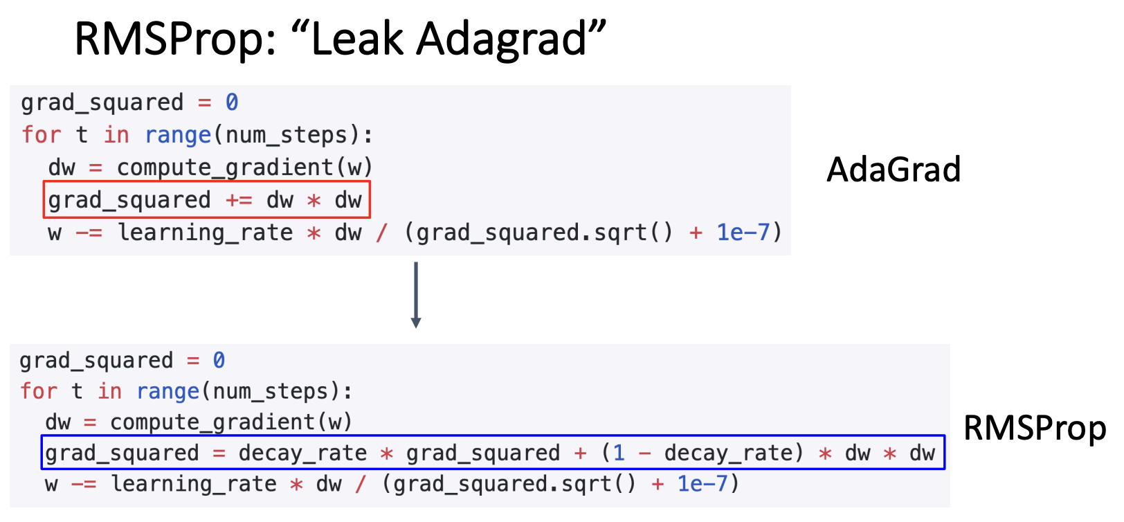
RMSProp is like to add extra friction with AdaGrad to decay our running average of square gradients.

Adam

We get two really good ideas in above parts, why not add them up?

Adam is basically RMSProp + Momentum.

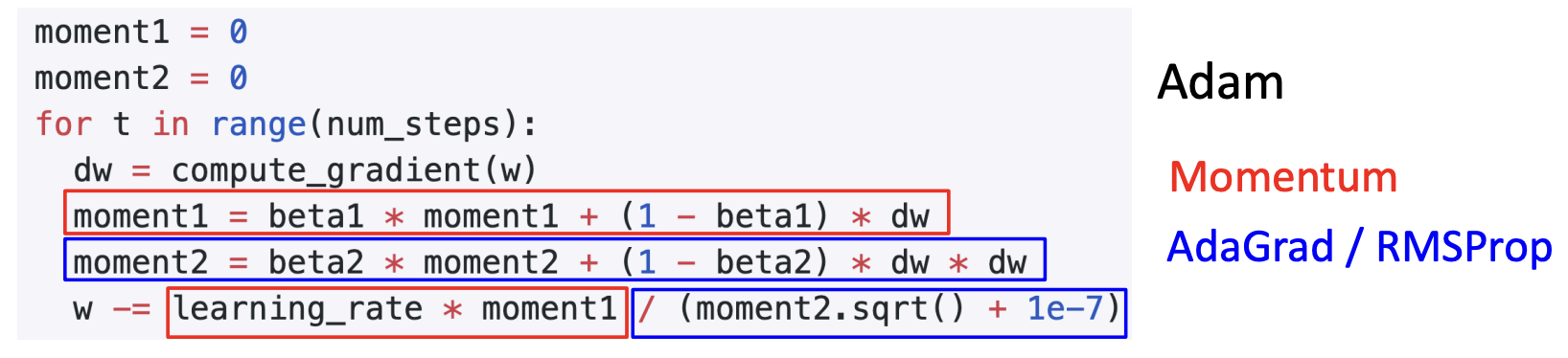
Q: What happens at t=0? (Assume beta2 = 0.999) moment2$\rightarrow$0 The Denominator of the last equation$\rightarrow$0 We end up taking a very very large gradient step at the very beginning of optimization.

The full from of Adam has the third good idea which is to add a bit of bias correction. Bias correction for the fact that first and second moment estimates start at zero.

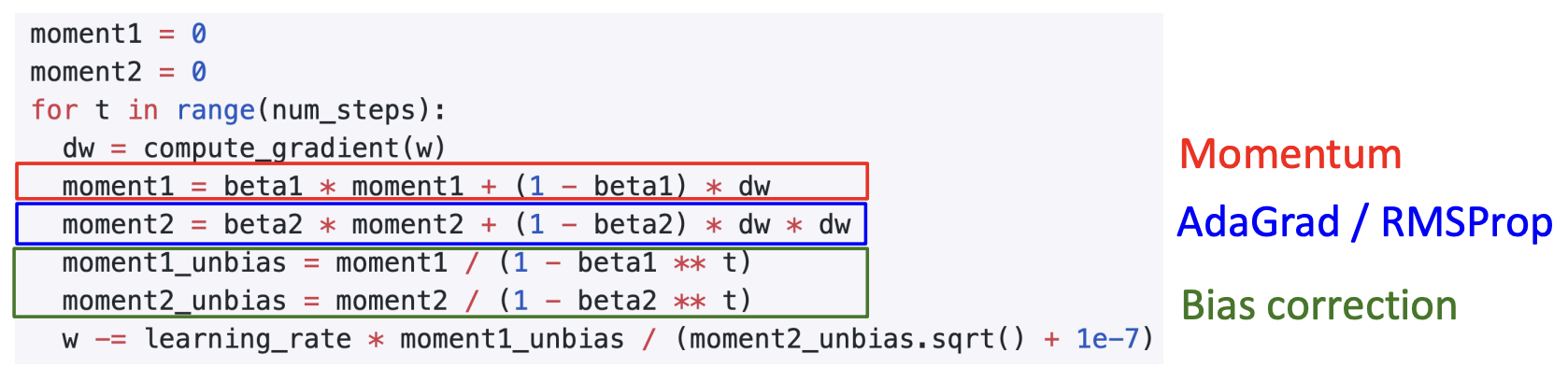
Adam with beta1 = 0.9, beta2 = 0.999, and learning_rate = 1e-3, 5e-4, 1e-4 is a great starting point for many models!

Conclusion

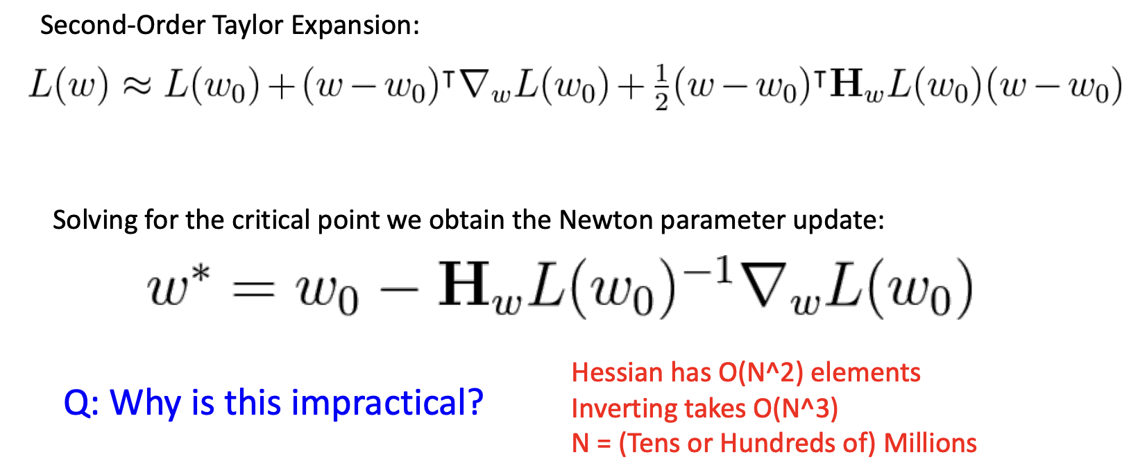
Second-Order Optimization

So far, we learn how to do the First-Order Optimization:

1. Use gradient to make linear approximation
2. Step to minimize the approximation

We can extend this thinkinf to use higher order gradient information.

For Second-Order Optimization:

1. Use gradient and Hessian to make quadratic approximation
2. Step to minimize the approximation

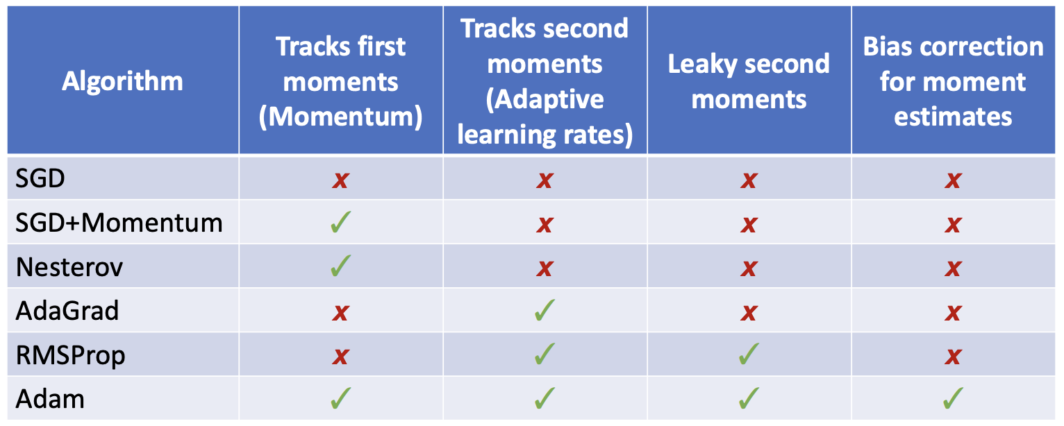
In practice:

• Adam is a good default choice in many cases; SGD+Momentum can outperform Adam but may require more tuning.